Linear to Exponential Voltage Conversion

Overview

Conversion from a linearly varying control voltage to an exponential current is a key building block for VCOs, VCFs, etc.: we perceive differences in audio signals in relative ratios (e.g. an octave is a doubling in $f_0$ ). There are a few references that this design is based on, and those are a good starting point to understand the circuit (see the References section below):

Hal Chamberlain's Musical Applications of Microprocessors. The section on the VCO includes this block, but if you can't find that book, ...
Rene Schmitz's "tutorial on exponential converters and temperature compensation", which goes into more detail on temperature compensation,
and finally, in an excellent lecture-style presentation, Aaron Lanterman's "Exponential Voltage-to-Current Conversion & Tempco Resistors" video.

In this note, I'm documenting the design steps for the core circuit, but will also collect other variations as I find them. The main thing I've added in these notes are derivations for including a normal resistor in parallel with the PTC thermistor in the feedback of the input gain stage, which can help approximate the desired thermal response when the classic 3300ppm/C thermistors are nowhere to be found.

Design

Differential Pair

The design starts with an NPN BJT differential pair.

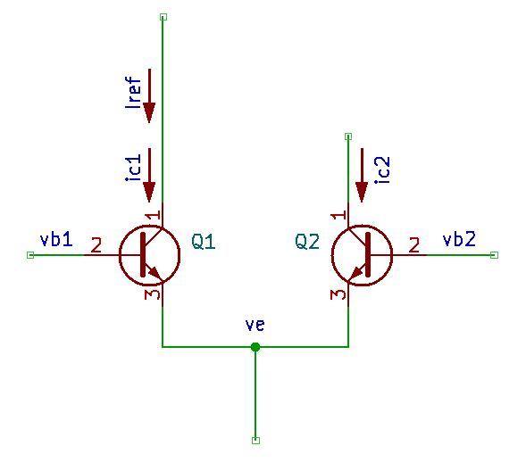
Using the relationship between $v_{be}$ and $i_c$ for an NPN BJT ( $i_c = I_S \exp\left(v_{be}/V_T\right)$ ) and assuming that the transistors are matched ( $I_{S1} = I_{S2}$ ), the collector current in Q2 ( $i_{c2}$ ) is related to the difference in the voltages at the bases when the emitters are at the same voltage $v_e$ :

$\begin{align*} \frac{i_{c2}}{i_{c1}} &= \frac{I_{S2}\exp\left(v_{be2}/V_T\right)}{I_{S1}\exp\left(v_{be1}/V_T\right)} \\ \to i_{c2} &= i_{c1}\exp \left(\frac{v_{b2} - v_{e} - v_{b1} + v_{e}}{V_T}\right) \\ &= i_{c1}\exp \left(\frac{v_{b2} - v_{b1}}{V_T}\right), \quad\mathrm{NPN} \end{align*}$

Grounding the base of Q2 sets $v_{b2} = 0$ and with $i_{c1} = I_{ref}$

$i_{c2} = I_{ref}\exp\left(-\frac{v_{b1}}{V_T}\right)$

Note

The choice of setting vb1 or vb2 to ground will change the sign on the input voltage, so inverting and non-inverting inputs can be constructed. The inverting input is useful when preceded by an inverting opamp buffer/sum.

When the NPN transistors are replaced with PNPs, the sign on $v_{be}$ is inverted: $i_c = I_S \exp\left(-v_{be}/V_T\right)$ (current flowing out of the collector). Taking the ratio of $i_{c2}/i_{c1}$ ,

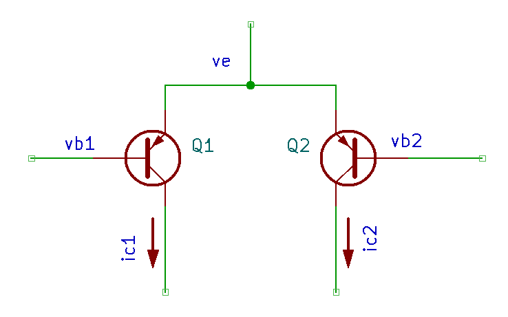
$\begin{align*} \frac{i_{c2}}{i_{c1}} &= \frac{I_{S2}\exp\left(-v_{be2}/V_T\right)}{I_{S1}\exp\left(-v_{be1}/V_T\right)} \\ \to i_{c2} &= i_{c1}\exp \left(\frac{v_{e} - v_{b2} - v_{e} + v_{b1}}{V_T}\right) \\ &= i_{c1}\exp \left(\frac{v_{b1} - v_{b2}}{V_T}\right), \quad\mathrm{PNP} \end{align*}$

To obtain the same inverting behaviour as in the NPN case, ground the base of Q2 for the PNP differential pair

$i_{c2} = I_{ref}\exp\left(-\frac{v_{b2}}{V_T}\right)$

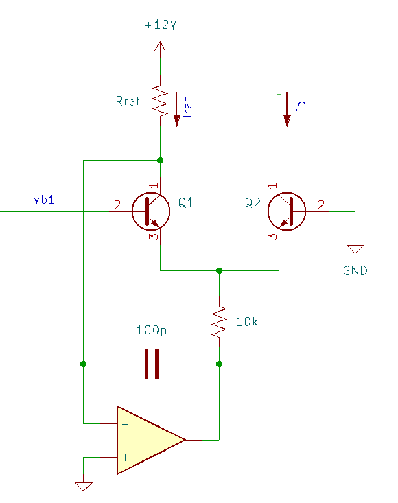
Returning to the NPN differential pair, the voltage difference across $R_{ref}$ sets the reference current $I_{ref} = i_{c1}$ . The voltage on the high side is set by the supply and on the low side by the op-amp, which replicates the reference voltage $V_n = 0$ at the non-inverting input to the collector of Q1. The circuit (described in [1]) is shown below:

Differntial pair with refernce current source

Input Stage Gain for V/Oct

To establish the desired gain of an input stage, let $v_{b1} = A v_{in}$ . When the input increases by 1V, the output current $i_p = i_{c2}$ should double:

$\begin{aligned} i_p &= I_{ref} \exp\left(-\frac{A v_{in}}{V_T}\right) \\ 2i_p &= I_{ref} \exp\left(-\frac{A (v_{in} + \Delta v_{in}}{V_T}\right) \\ \to \frac{2 i_p}{i_p} = 2 &= \exp\left(-\frac{A \Delta v_{in}}{V_T}\right) \\ \to \ln 2 &= -\frac{A \Delta v_{in}}{V_T} \\ \to A &= -\frac{V_T \ln 2}{1} = 0.693 V_T \approx -0.018 = -\frac{1}{55.5} \end{aligned}$

The value of $i_{p}$ will be equal to $I_{ref}$ when $v_{in}$ is at its minimum. This will set the smallest current.

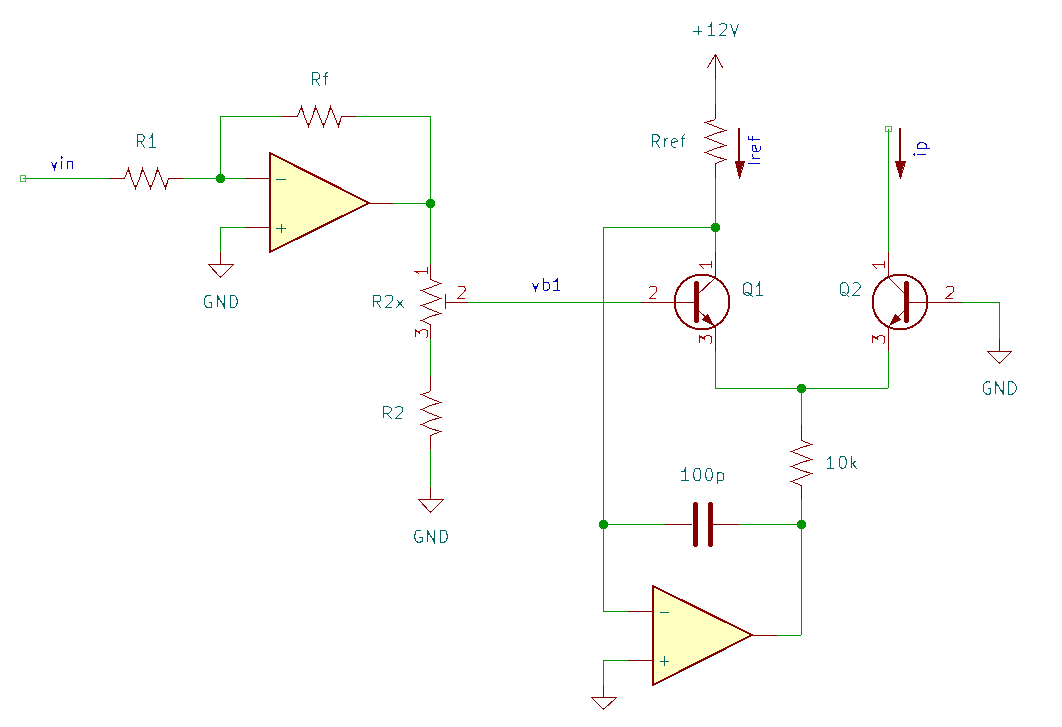
An op-amp in an inverting gain configuration with a voltage divider supplies $v_{b1}$ .

$\begin{aligned} A &= -0.693 V_T = -0.018 \simeq -\frac{1}{55.5} = -\frac{R_f}{R_1} \frac{R_2 + \alpha R_{2x}}{R_2 + R_{2x}} \\ \to \frac{1}{55.5} &= \frac{2\mathrm{k}\Omega}{100\mathrm{k}\Omega} \frac{440\Omega}{490\Omega} \end{aligned}$

where $R_{2x}$ is adjusted such that the voltage divider gives a gain of $0.9$ . The choice of $R_f = 2\mathrm{k}\Omega$ comes from a "common" (50 years ago) value of positive-temperature coefficient (PTC) resistors (details in the next section). Multiple inputs can be summed via $100\mathrm{k}\Omega$ input resistors. The voltage divider typically consists of a fixed $390\Omega$ resistor and a $100\Omega$ trim pot, enabling tuning to get V/Oct behaviour.

Current source with input stage

Temperature Compensation

Continuing with Lanterman's derivation, replace $R_f$ with a PTC resistor, $R_f = R_0[1+\alpha(T-T_0)]$ where $\alpha$ is the thermal coefficient (note: use $A'$ in place of $\tilde{\mathfrak{s}}$ ). The "P" in PTC is important: the resistance must increase with increasing temperature.

$\begin{aligned} A = -\frac{R_f}{R_1}A' &= -\frac{R_0[1+\alpha(T-T_0)]}{R_1}A' = -\underbrace{0.693}_{B} V_T \\ \to \frac{R_0[1+\alpha(T-T_0)]}{R_1}A' &= \frac{kT}{q}B = \frac{k[T_0 + (T-T_0)]}{q}B \\ &= \underbrace{\frac{kT_0}{q}}_{V_{T0}}B + \frac{kT_0}{q}\frac{(T- T_0)}{T_0}B \\ \to \frac{R_0}{R_1}A' + \frac{\alpha R_0 (T-T_0)}{R_1}A' &= \underbrace{V_{T0}B}_{A_0} + \frac{V_{T0}}{T_0}B (T- T_0) \\ \mathrm{let}\quad A_0 &\equiv \frac{R_0}{R_1}A' = V_{T0}B \\ \to \frac{\alpha R_0 (T-T_0)}{R_1}A' &= A_0 \alpha(T-T_0) = \underbrace{V_{T0}B}_{A_0}\frac{1}{T_0}(T- T_0) \\ \to \alpha &= \frac{1}{T_0} = 0.0034 \end{aligned}$

Note that the temperature coefficient is positive. It\'s hard to find 3300ppm tempco resistors in 2025, so here\'s an alternative derivation where $R_f = R_{f1}\parallel R_{f2}$ where $R_{f1}$ is a tempco resistor and $R_{f2}$ is a regular resistor (assumed constant in temperature).

$\begin{aligned} R_{f1}\parallel R_{f2} &= \frac{R_{f1}R_{f2}}{R_{f1} + R_{f2}} \\ &= \frac{R_0[1+\alpha(T-T_0)]R_{f2}}{R_0[1+\alpha(T-T_0)] + R_{f2}} \\ &= R_0\frac{1 + \alpha(T-T_0)}{\frac{R_0}{R_{f2}}[1+ \alpha(T-T_0)] + 1} \\ &= R_0\frac{1 + \alpha(T-T_0)}{\left(1 + \frac{R_0}{R_{f2}}\right) + \underbrace{\frac{R_0}{R_{f2}}\alpha}_{\alpha'}(T-T_0)} \\ \end{aligned}$

Assuming $\alpha'(T-T_0) \ll 1$ (prefer $R_{f2} > R_0$ )

$\frac{1}{p + \alpha(T-T_0)} \approx \frac{1}{p} - \frac{\alpha(T-T_0)}{p^2}$

such that

$\begin{aligned} R_{f1}\parallel R_{f2} &\approx R_0\left[1 + \alpha(T-T_0)\right]\left(\frac{R_{f2}}{R_0 + R_{f2}}\right) \left[ 1 - \frac{R_{f2}\alpha'(T-T_0)}{R_0 + R_{f2}}\right] \\ &= \left(\frac{R_0 R_{f2}}{R_0 + R_{f2}}\right)\left[1 + \alpha(T-T_0)\right] \left[ 1 - \underbrace{\frac{R_0}{R_0 + R_{f2}}}_{\gamma}\alpha(T-T_0)\right] \\ &= \left(\frac{R_0 R_{f2}}{R_0 + R_{f2}}\right)\left[1 + \alpha(T-T_0)\right] \left[ 1 - \gamma\alpha(T-T_0)\right] \\ &= \left(\frac{R_0 R_{f2}}{R_0 + R_{f2}}\right)\left[1 + (1-\gamma)\alpha(T-T_0) - \gamma\alpha^2(T-T_0)^2\right]\\ \end{aligned}$

Given an available PTC resistor with resistance $R_0$ and temperature coefficient $\alpha_0 > \alpha = 0.0034$ , the parallel resistance $R_{f2}$ can be found as

$\begin{aligned} \alpha &= (1-\gamma)\alpha_0 = \left(1 - \frac{R_0}{R_0 + R_{f2}}\right)\alpha_0 \\ \to \frac{R_0}{R_0 + R_{f2}} &= 1 - \frac{\alpha}{\alpha_0} \\ \to \frac{R_0\alpha_0}{\alpha_0 - \alpha} &= R_0 + R_{f2} \\ \to R_{f2} &= R_0\left(\frac{\alpha_0}{\alpha_0 - \alpha} - 1\right) = R_0\left(\frac{\alpha}{\alpha_0 - \alpha}\right) \end{aligned}$

There is a calculator for $R_{f2}$ and $R_0$ in this notebook.

The following table collects a few currently manufactured parts available on Digikey (as of 2025):

Mfg.	Part #	Package	$R_0\ (\mathrm{k}\Omega)$	$\alpha (\mathrm{ppm/K})$
KOA Speer	LT732ATTD202J3900	0805	2	3900
KOA Speer	LT732ATTD102J3600	0805	1	3600
Vishay Dale	TFPT1206L1002FM	1206	10	4110
Vishay Dale	TFPTL15L5001FL2B	THT 2.5mm	5	4110
Texas Instruments	TMP6131LPGM	TO90-2	10	6400

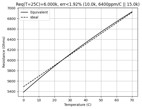
As an example, the TMP6121LPGM (10k, 6400ppm/C TCR with 1% tolerance) in parallel with a 15k resistor approximates a 6k resistor with a 3400ppm/C temperature with a maximum error of less than 2% over the range from 0-70C.

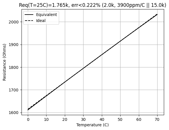
A second example is the LT732ATTD202J3900 (2k, 3900ppm/C TCR with 10% tolerance) in parallel with a 15k resistor. This configuration approximates a 1.765k resistor with a 3400ppm/C TCR to less than 0.3% over the range from 0-70C.

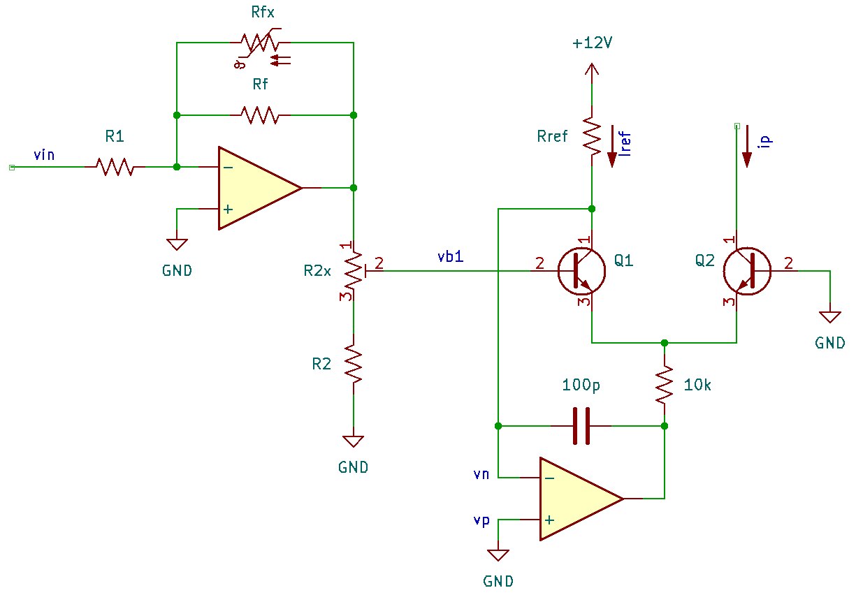
With $R_{f}\parallel R_{fx} = 1.765\mathrm{k}\Omega$ (2k PTC thermistor in parallel with a 15k resistor), $R_1 = 82\mathrm{k}\Omega$ gives an approximate gain in the inverting amplifier of $0.0215$ per the design requirement (the remaining fraction can be tuned in a $100\Omega$ trim pot in series with a $220\Omega$ resistor in the voltage divider -- note that this is different than the classic 100+390 pair).

A schematic of the complete block is shown below.

References

Hal Chamberlain, Musical Applications of Microprocessors, 2nd Ed., Hayden Books, 1985
Rene Schmitz, "A tutorial on exponential converters and temperature compensation", [schmitzbits.de]
Aaron Lanterman, "ECE4450 L18: Exponential Voltage-to-Current Conversion & Tempco Resistors", [youtube]
Paul Horowitz and Winfield Hill, The Art of Electronics, 3rd Ed., Cambridge University Press, 2015